With VMware jacking up the prices and killing off the free version of ESXi, people are looking to alternatives for a virtualization platform. One of the more popular alternatives is Proxmox, which so far I’m really liking.
If you’re looking to run CVP on Proxmox, here is how I get it installed. I’m not sure if Proxmox counts as officially supported for production CVP (it is KVM, however), but it does work fine in lab. Contact Arista TAC if you’re wondering about Proxmox suitability.
Getting the Image to Proxmox
Oddly enough, what you’ll want to do is get a copy of the CVP OVA, not the KVM image. I’m using the most recent release (at the time of writing, always check Arista.com) of cvp-2024.1.0.ova.
Get it onto your Proxmox box (or one of them if you’re doing a cluster). Place it somewhere where there’s enough space to unpack it. In my case, I have a volume called volume2, which is located at /mnt/pve/volume2.
I made a directory called tmp and copied the file to that directory via SCP (using FileZilla, though there’s several ways to get files onto Proxmox, it’s just a Linux box). I then untared the OVA with tar -xvf (I know, right? I had no idea it was just a tgz ball).
root@proxmox:/mnt/pve/volume2/tmp# tar -xvf cvp-2024.1.0.ova
cvp.ovf
cvp.mf
cvp-disk1.vmdk
cvp-disk2.vmdk
In my case, this gave me four files, two of which are vmdk disk files.
Importing the OVA to Proxmox Inventory
The next step is to import the disks and the VM into system inventory. You’ll need to pick a volume to place it in, as well as a unused VMID. In my case, I’m using volume2 and the VMID of 109, which was available in my environment.
root@proxmox:/mnt/pve/volume2/tmp# qm importovf 109 cvp.ovf volume2 --format qcow2
...
transferred 0.0 B of 1.0 TiB (0.00%)
transferred 11.0 GiB of 1.0 TiB (1.07%)
transferred 21.8 GiB of 1.0 TiB (2.13%)
transferred 32.8 GiB of 1.0 TiB (3.20%)
transferred 43.7 GiB of 1.0 TiB (4.27%)
...
This process will take a few minutes at least. You’ll see it refer to 1 TiB, but don’t worry, it’s thin provisioned so it’s not actually going to take up 1 TB (at least not initially).
You should now see the VM in your Proxmox Inventory. I would change the name, as well as up the RAM to something higher (it starts with 28 GB, I put it at around 36 GB of RAM). You’ll need to add a NIC as well. Put it on a virtual switch (bridge) and select VirtIO for the NIC model.
From there you can follow the install CVP instructions. Remember you’ll need both forward and reverse DNS records, as well as access to an NTP server to complete the install.
Ansible is a great platform for network automation, but one of its quirks is its sometimes obtuse errors. I was running a playbook which logs into various Arista leafs and spines and does some tests. I’m using SSH to issue the commands (versus eAPI). I got this error:
fatal: [spine1]: FAILED! => {"changed": false, "msg": "Connection type ssh is not valid for this module"}
One of the little things that trips me up when doing Ansible with network automation is the connection type.
When you’re automating servers (Ansible’s original use case) the connection type is assumed to be SSH, so the Ansible control node will log in to the node and perform some functions. The default connection type is “ssh”.
It’s a little counter-intuative, but even if you’re using SSH to get into network device, most network-centric modules won’t work. You need to use another connection type such as network_cli, which is part of the netcommon module collection. When you use network_cli, you also might have to specify a few other options such as network_os, become, and become_method.
        ansible_connection: network_cli
        ansible_network_os: eos
        ansible_become: yes
        ansible_become_method: enable
If your device has some sort of API, you can use httpapi as the connection type. You’ll almost always need to specify to use SSL and to set validate_certs to false (as in most cases devices have a self-signed certificate).
        ansible_connection: httpapi
        ansible_httpapi_use_ssl: True
        ansible_httpapi_validate_certs: False
        ansible_network_os: eos
        ansible_httpapi_port: 443
There’s also netconf and a few others.
So whether your network device is controlled via SSH/CLI or some type of API (JSON-RPC, XML-RPC, REST) make sure to set the connection type, otherwise Ansible probably won’t work with your network device.
When choosing an underlay for an EVPN/VXAN network, the prevailing wisdom is that BGP is the best choice for the underlay routing protocol. And overall, I think that’s true. But OSPF can make a compelling underlay too, as it has a few logistical advantages over BGP in certain cases.
When building out EVPN/VXLAN networks, I like to break the build into four components. They are layers that are built one-by-one on top of each other.
Topology (typically leaf/spine)
Underlay (provides IP connecitivity for loopbacks)
Overlay (exchanges EVPN routes)
EVPN services (these are the Layer 2 and Layer 3 networks internal hosts and external networks connect to)
This article is exclusively about the underlay portion. It’s a very simple routed network that has one job, and job only:
Provide routes to enable IP connectivity from any loopbacks on a device to any loopback on any other device.
That’s it.
In normal operation the routing table will be incredibly static. The only time the routing table would change is when a switch is added or removed, or a link goes down, or a switch is upgraded, etc. In regular operation it won’t change.
The underlay is important, but the underlay isn’t complicated.
You have a number of routing protocols to choose from to enable this. Technically any routing protocol (or even static routes!) would work, but the most common and sensible routing protocols are as follows:
BGP (eBGP or iBGP, depends on your overlay)
OSPF
ISIS (to a lesser extent)
I even built a working underlay with RIP, though its lack of ECMP would preclude it from being used. I just did it to see if it could be done. Don’t use RIP, kids.
BGP and OSPF are the most common underlays. ISIS can be used, but ISIS is not a skillset that’s terribly common in the DC. So let’s talk about the two remaining choices: OSPF and BGP.
For any kind of EVPN/VXLAN fabric, BGP has no scaling issues, so you can scale up to as many nodes as you dare have in a single failure domain.
For smaller scales and labbing, I generally don’t like BGP as the underlay. Here’s a few reasons I prefer OSPF for some smaller-scale environments and labs:
IP unnumbered (not needing IP addresses on the point-to-point links)
Stupidly simple routing protocol configuration (just set everything to area 0 and set a router-id)
Separation of function: BGP handles the overlay (EVPN routes) and OSPF handles the underlay
Separation of Function
When I was learning EVPN/VXLAN I made sure to put OSPF as an underlay. I knew it well enough to do the job it was intended for, and I was less confident with BGP. It really helped to have BGP only be involved with the overlay. As I was playing with settings, figuring out what was required and not required, how everything behaved… it really helped to know that anything under “router bgp” was EVPN.
In certain production environments this may also be advantageous, especially for smaller organizations that are just getting up to speed with EVPN/VXLAN. It can make troubleshooting a bit easier.
IP Unnumbered
I love IP unnumbered. As an instructor, I do a lot of EVPN configuration demonstrations. In front of the students I will build, by hand, a soup-to-nuts EVPN/VXLAN network. Of course, EVPN/VXLAN in production should almost always be configured through automation (specifically configuration generation, assuming the switches use config file), but for labbing you’re going to do it manually. You have to understand how to do something manually before automation/troubleshooting it.
BGP, being TCP-based, requires an IP address in order to peer with another device. This typically means you’ll have to come up with an IP scheme of point-to-point IP addresses between every leaf and spine. With three spines and four leafs, that’s 24 unique IP addresses that need to be assigned total, two per each each leaf-to-spine link. With three spines and 20 leafs, that’s 60 unique IPs. This isn’t horrible by any means, but it’s a pain.
Here’s an example of the configuration for point-to-point interface configurations between an Arista EOS leaf and spine:
LEAF1
interface Ethernet3
  ip address 192.168.103.0/31
  no switchport
  mtu 9214

SPINE1
interface Ethernet1
  ip address 192.168.103.1/31
  no switchport
  mtu 9214
And those IPs need to be plugged into the BGP configuration:
router bgp 65101
...
   neighbor 192.168.103.1 peer group Underlay
   neighbor 192.168.103.3 peer group Underlay
   neighbor 192.168.103.5 peer group Underlay
So with BGP as an underlay, a significant portion of the underlay configuration will be unique to each leaf/spine. If you’re doing this by hand, it’s easy to make a mistake with all of those /31s. This alone is one of the reasons one should only configure EVPN/VXLAN in production using automation.
You’ll also want to do something to keep the /31s out of the routing tables, such as route-maps, otherwise the /31s get everywhere and they’re not needed. They’ll eat up forwarding table space (not a super big deal, but still) and crowd a “show ip route”.
With OSPF, the situation is much more simplified. The interface configurations are the same for all p2p links by using ip unnumbered:
interface Ethernet2
  no switchport
  ip address unnumbered loopback0
  ip ospf area 0
  ip ospf network point-to-point
  mtu 9214
With OSPF, a neighbor adjacency can be brought up without an individual IP address. As for the OSPF protocol configuration, usually all you need to do is setup the router-id (always set up the router-id). The following is all that’s required:
router ospf 10
  router-id 1.1.1.1 <--- this is usually the loopback0 address
Very simple, and very repeatable (when compared to BGP as the underlay).
Of course most of the automation platforms will do this for you. For example, Arista AVD and Arista CloudVision Studios will generate the p2p IPs from a block of addresses you specify. But if you’re labbing with manual configuration or rolling your own automation (such as Ansible/Jinja templates) this can complicate matters.
But “IPv6 Unnumbered”?
The ability to use “IPv6 unnumbered” does simplify things a little bit, as using rfc 5549 doesn’t require assigning IP addresses to the p2p interfaces. Technically it’s not unnumbered, but instead makes use of the link local address and neighbor discovery aspects of IPv6.
#show ip bgp summary <--- showing the underlay routing protocol
BGP summary information for VRF default
Router identifier 192.0.200.3, local AS number 65101
Neighbor Status Codes: m - Under maintenance
Description   Neighbor                        V AS      MsgRcvd   MsgSent  InQ OutQ  Up/Down State   PfxRcd PfxAcc
  spine1      fe80::20c:73ff:fe10:335d%Et3    4 65001         8        11    0    0 00:01:55 Estab   4      4
  spine2      fe80::20c:73ff:fe76:1b6b%Et4    4 65001         8        11    0    0 00:01:56 Estab   4      4
  spine3      fe80::20c:73ff:fefd:a9d8%Et5    4 65001         9         9    0    0 00:01:56 Estab   4      4
On the p2p interace you must enable ipv6, and the switch will auto-assign a link-local IPv6 address.
interface Ethernet3
   description P2P_LINK_TO_SPINE1_Ethernet2
   no switchport
   ipv6 enable
And in the BGP configuration rather than specifying the neighbor IP address, you just specify the interface and the NOS will auto-find the peer IP.
You can see the link-local IPv6 address that the interface chose:
1#show ipv6 interface brief
   Interface       Status        MTU       IPv6 Address                     Addr State    Addr Source
--------------- ------------ ---------- -------------------------------- ---------------- -----------
   Et3             up           1500       fe80::21c:73ff:fe32:7cb/64       up            link local
So that does get rid of the complexity of assigning IPs to p2p links, though there’s still more simplicity in OSPF configurations.
Stupid Simple
OSPF has another advantage as an underlay: It’s incredibly simple. It has everything you want in an underlay with the only knob you need to touch is setting the router id. ECMP, clutter-free routing tables, loopback-to-loopback connectivity is there with the defaults. Just throw everything in area 0 and set the router-id, set the interfaces to unnumbered and point-to-point, and that’s it.
When you’re starting out on your learning EVPN journey, or for smaller organizations, this can be huge benefit.
BPG is more customizable of course, but for an underlay there’s usually no need for customization. We want the simplest, most symmetrical network possible.
The Cases Against OSPF
There are a few cases against OSPF as an underlay. In all cases with EVPN, the overlay (exchanging endpoint information, external networks, etc.) is done with BPG. Specifically, MP-BGP (either iBGP or eBGP can be used). But as we’ve shown, the underlay is up for grabs. So why not use OSPF?
The biggest issue I think is scale. Or rather, concern about scale. There’s been enough large implementations of BGP that we don’t really worry about its scale. But there has historically been concern and assumptions about OSPF scaling. Here’s an article talking about large scale Clos networks with OSPF as the routing protocol.
Given the stability, simplicity, and relatively small size of the routing table of most underlay networks, I think that OSPF is fine for a small to medium sized environment. For larger environments, you could probabably do multi-areas for various leaf/spine groups connected to super spines on area 0, etc. But at that point you might as well do BPG on the underlay, as at that size you’ll have a pretty sophisticated automation system.
Automation systems level the playing field with underlay routing protocols for the most part. If you’re making your own automation system using Jinja and Ansible, for instance, OSPF makes some of that easier. But if you’re using a pre-made system like I mentioned before, such as Arista AVD, the difference between OSPF and BPG in the underlay is as simple as a key value pair in a data model.
TL;DR
So here’s the too-long, didn’t read: For labbing, use OSPF. If you’re making your own templates in Jinja and Ansible, OSPF probably is easier until you hit a certain scale. If you’re using a pre-made automation system, just use what’s easiest (probably BGP). Automation can erase and difference between complexity of one versus the other.
TL;DR: If you’re a sysadmin or network administrator who doesn’t know vi/vim, I wouldn’t worry about it. Nano as a Linux/Unix editor will suffice in just about every situation you’re likely to be involved in.
Vi (and its successor, vim) is a text editor commonly used on Unix-like systems like Linux, the BSDs, and MacOS (I’m not getting into a what is/isn’t Unix discussion). If it’s remotely Unix-like, typing “vi” will likely get you vi, vim, or another variant. You can pretty much count on vi being there.
When I started as a Unix admin back in the 1990s, primarily working with Solaris and SunOS, knowing your way around vi is what I would classify as an essential skill. The other editors were pico (easy to learn) and Emacs (very high learning curve). Vi versus Emacs was one of the first technology “religious” wars.
I don’t have much experience with Emacs. I gave it a go in the late 1990s at one point, but found the learning curve too discouraging. Besides, I could already do everything I needed to with vi and Emacs users didn’t seem to be able to do something I couldn’t do. It felt like to me (at the time at least) that the learning curve for Emacs was higher than vi, but that’s a pretty subjective call.
The reasons why I don’t think it’s necessary to learn vi today is based on what we used it for, versus what we need today. So what did we use these editors for?
In the 1990s, servers were bespoke, artisanal, and one of a kind. They were “pets” in the pets vs cattle parlance. You would install a server manually, configure it manually, deploy services on it manually, and maintain it manually. It was common to compile your own Apache and MySQL, for example. All if this involved editing various files. Make files, config files, network ini files, and whatever level of hell that sendmail config files were. For these types of environments, vi was an invaluable tool. The various configurations files (especially the insane configs of sendmail) could be quickly edited. With a few keystrokes you could open a huge config file, page up and down, go to any line number, search for the right parameter, replace it, save, and exit. There was mass search and replace and a lot of tools that we take for granted in a GUI-based editor but didn’t exit in the basic command line text editors.
So if you were slinging servers for a living, vi/vim were invaluable tools.
If you were writing software, vi was a great editor and vim brought color schemes, which would apply one color to variables, another to functions, etc. I did a bit of Bash and Perl for server automation and PHP for some dynamic website tools. Vi/vim was great for this.
But the world of server administration is very different today than it was in the 1990s. Manual configuration is much more limited, instead best practices usually involve some sort of automation such as Ansible. Writing scripts and now playbooks are typically done off a server by some sort of IDE, most notably now VS Code from Microsoft. Same for any kind of software writing.
Any editing that’s done on an actual server is typically very minimal, so the benefits of vim don’t really provide a lot of value. At least it doesn’t provide nearly the return on investment that it did in the 1990s.
Instead, if you find yourself needing to edit on-system, I recommend using the nano editor. Nano is the successor to pico, and is a fairly basic text-based editor. For editing a configuration file or some other text file on a Linux machine or other Unix-like system it’s more than sufficient and can be used without any training.
I’m not discouraging anyone from using vi, Vim, or even Emacs. I’m not even discouraging really anyone from learning those tools. I’m just saying that in a world of lots of stuff to learn I don’t consider them must-needed skills for your typical networking admin or server admin.
“It’s all fun and games until you can’t ping your default gateway.”
While EVPN/VXLAN brings a number of benefits when compared to a more traditional Core/Aggregation/Access layer style network with only VLANs and SVIs, it is different enough that you’ll need to learn some new troubleshooting techniques. It’s not all that different than what you’ve probably done before, but it is different enough to warrant a blog post.
This article is on how to troubleshoot EVPN/VXLAN on Arista EOS switches, and the command line commands will reflect that. However, as EVPN/VXLAN are a collection of IETF standards, the overall technique will translate to any EVPN/VXLAN platform.
The scenario this article is going to explore is endpoint to endpoint connectivity, though it can also be easily modified for endpoint to network connectivity. It doesn’t matter if the host is on the same VXLAN segment or a different one.
The primary strategy will be to verify the control plane. EVPN/VXLAN has a control plane, a data plane, an overlay and an underlay. Generally, I’ve found that most issues occur on the control plane. The control plane process looks like this:
MAC address is learned on the ingress leaf VLAN
MAC learning triggers creating of Type 2 routes (a MAC route and a MAC-IP route)
Type 2 routes are propagated to all other switches in the fabric (including the egress leaf)
Type 2 routes are installed into the appropriate forwarding tables (Layer 2, Layer 3) on the egress leaf
While this method only verifies the control plane, going through this list one by one should expose any issues with the underlay or overlay. If the issue still isn’t identified, verification can move to the data plane which will be covered in a different article. We’re staring with the control planes as if the control plane hasn’t told the data plane how to forward, the data plane can’t forward.
Here’s a couple of things to keep in mind with EVPN/VXLAN
You need the MAC address of the endpoint in question to start. This all flows from the MAC address. Other information from the endpoint, such as ARP table (do we have the MAC of the default gateway?), default gateway and any static routes, and even link status (is it even plugged in/connected to a virtual port on a virtual switch?)
All leafs and spines (and superspines) will have every EVPN route. They don’t all need to install the routes into a forwarding table, but they will have every EVPN (type 2, type 3, etc.) route. If they don’t, that means something is likely wrong.
Every VXLAN segment requires a local VLAN to be connected do it.
The Hypothetical Environment
The physical connectivity is listed here below. There’s two hosts, on two different segments.
In this hypothetical environment, there are two hosts that can’t communicate. Host1 is on L2VNI 10010, and Host2 is on L2VNI 10020. There is symmetric IRB, with a L3VNI for the VRF of 10000.
It’s important to know the logical layout (L2VNIs, IP-VRF, etc.) before starting.
Endpoint MAC/IP (source)
Local VLAN ID
VXLAN ID (L2VNI)
IP-VRF
L3VNI for IP-VRF
Egress VXLAN ID (may or may not be different)
Egress VLAN ID (may or may not be different)
Endpoint MAC/IP (destination)
For this exercise, here is that information:
0000.0000.0001 and 10.1.10.11/24
VLAN 10
VNI 10010
VRF: Red, L3VNI 10000
VNI 10020
VLAN 20
0000.0000.0002 and 10.1.20.12/24
A Note On The Non-Network Team Environment
As is often the case, the packets from the host may traverse configuration domains outside of the network team’s purview. Most commonly these are virtual switches and blade switches. Ideally the network team would at least have read-only access to these environments, but that’s not always possible.
Hopefully the teams responsible for these environments can check to see the MAC address of the host ended up in the appropriate forwarding tables. For example, the port group on the hypervisor in VMware has a way to check MAC addresses. Cisco UCS, a popular blade system, also has a way to see the MAC addresses learned on the switch (the command is the same as on EOS, in fact).
The Strategy
The diagram below shows the strategy, starting from the ingress leaf to the egress leaf. Normally the hosts would be connected to multiple leafs in either MLAG or EVPN multihoming, but to simplify things this scenario involves two single-homed hosts. Everything will be working correctly, so no issues will be found in the verification as to show you what it should look like.
In addition, the EOS configuration relevant to the verification will be shown.
MAC Address Learned on the Ingress Leaf
This is fairly straightforward, and the verification is the same as you’d be used to in a more traditional network. You’ll want to know the VLAN and VXLAN segment it’s assigned to. You should see the host’s MAC in the local leaf’s MAC table. If you don’t, that needs to be resolved before you can continue. Nothing will work unless the ingress leaf sees the MAC address.
You’ll have to generate some type of traffic of course for the MAC address to be learned. Running a constant ping from the host will do it, or you can also setup (or pre-stage in a tightly change controlled environment) a diagnostic loopback in the Tenant VRF to ping from the leaf to the host.
The command is show mac address-table vlan 10 in this case.
leaf1#show mac address-table vlan 10
          Mac Address Table
------------------------------------------------------------------

Vlan    Mac Address       Type        Ports      Moves   Last Move
----    -----------       ----        -----      -----   ---------
10      0000.0000.0001    DYNAMIC     Po67       1       0:00:56 ago
Total Mac Addresses for this criterion: 1
The configuration that enables this is below:
interface Ethernet6
   channel-group 67 mode active
interface Ethernet7
   channel-group 67 mode active
interface Port-Channel67
   switchport access vlan 10
Type 2 Route Generation
So the MAC address was learned on the correct VLAN. We can move onto the next step, which is to see if learning the MAC address generated Type 2 routes. Because we’re routing from one VXLAN segment to another VXLAN segment, there will two EVPN Type 2 routes created: One for the MAC address and one for the MAC and IP combination.
The command to see these routes is show bgp evpn route-type mac-ip. You can optionally specify the MAC address, which can be useful is there’s a lot of endpoints in the routing table.
#show bgp evpn route-type mac-ip 0000.0000.0001
BGP routing table information for VRF default
Router identifier 192.168.101.11, local AS number 65101
Route status codes: s - suppressed, * - valid, > - active, E - ECMP head, e - ECMP
                    S - Stale, c - Contributing to ECMP, b - backup
                    % - Pending BGP convergence
Origin codes: i - IGP, e - EGP, ? - incomplete
AS Path Attributes: Or-ID - Originator ID, C-LST - Cluster List, LL Nexthop - Link Local Nexthop

          Network                Next Hop              Metric  LocPref Weight  Path
 * >     RD: 192.168.101.11:10010 mac-ip 0000.0000.0001
                                 -                     -       -       0       i
 * >     RD: 192.168.101.11:10010 mac-ip 0000.0000.0001 10.10.10.11
                                 -                     -       -       0       i
This switch has generated two type 2 routes: One for the MAC address by itself, and one for the combination of MAC and IP. For symmetric IRB (the most common EVPN configuration) this will be the case. Normally a VLAN just learns the MAC address, but with EVPN the VLAN also learns the IP address if the initial frame contains that information (it would in an ARP, for instance).
MP-BGP with the EVPN address family is responsible for generating these routes based on MAC and IPs learned in a VLAN. There are two common ways to configure a leaf to generate Type 2 routes for a VLAN/VNI: Individually or in bundles. They’re called VLAN services or VLAN-aware bundle services.
Below is what the configuration would look like for an individual VLAN service for two VLANs:
Note that each VLAN has its own route distinguisher and its own route target.
For VLAN aware bundles, all the VLANs in a Tenant can be placed into a single instance:
router bgp 65101
  ...
  vlan-aware-bundle Red
    rd 192.168.101.1:1000
    route-target both 1000:1000
    redistributed learned
    vlan 10,20
Route Propagation to Spines
The route generated on the ingress leaf should propagate to the connected spines, and from there all other leafs and perhaps superspines. They won’t necessarily be installed into any forwarding tables (for example, they won’t be installed on the spines), but they should be on all fabric switches, regardless of role.
The next step is to verify that the route made it to the spine. Log into one of the spines and run the same show command, show bgp evpn summary.
If MLAG is being used, you’ll see the same two routes twice: One from each leaf in the MLAG group. They will be differentiated by their route distinguishers.
If they’re not on the spines, resolve that before continuing. This is entirely configured in the overlay configuration and underlay. I would check the overlay first, then the underlay to resolve any reasons that the routes aren’t being propagated. If the routes aren’t making it to the spines connected to the ingress leaf, then none of the other leafs will get those routes and won’t know what to do with packets destined for that MAC or IP.
Egress Leaf
The routes should make it to the egress leaf. To verify, it’s the same show bgp evpn route-type mac-ip command. You will see the same routes multiple times. For instance, if you have one ingress leaf and three spines, you’ll see the MAC and MAC-IP routes both three times each. One MAC route each from three spines, one MAC-IP route each from three spines.
If the egress leafs are in an MLAG pair, you’ll see even more. Two leafs, two route types, three spines: You’ll see 12 routes for the endpoint. That’s normal. Note the routes all point the same VTEP in this example (192.168.102.11).
Now that the egress leaf has the routes, it can program them into the forwarding tables. For EVPN, that can mean either the IP VRF or the VLAN forwarding table (or both).
If the ingress VXLAN segment isn’t configured to a VLAN on the egress leaf, then the MAC address won’t go into a VLAN. That’s normal. However, if the VXLAN segment is configured for a local VLAN, you can verify the route was programmed with a simple show mac address-table vlan. Also you can run show vxlan address-table.
#show mac address-table vlan 10
Mac Address Table
------------------------------------------------------------------
Vlan Mac Address Type Ports Moves Last Move
---- ----------- ---- ----- ----- ---------
10 0000.0000.0001 DYNAMIC Vx1 1 0:01:13 ago
Total Mac Addresses for this criterion: 1
#show vxlan address-tablevlan 10
Vxlan Mac Address Table
----------------------------------------------------------------------
VLAN Mac Address Type Prt VTEP Moves Last Move
---- ----------- ---- --- ---- ----- ---------
10 001c.73cd.693d EVPN Vx1 192.0.254.3 1 0:05:18 ago
Total Remote Mac Addresses for this criterion: 1
The egress host in the example is on another VXLAN segment/VLAN, however. For 10.1.20.12 to get to 10.1.10.11, there would need to be a /32 host route in the IP VRF. You can see this with a show ip route vrf [IP-VRF]. In this case, the IP VRF is “Red”.
#show ip route vrf Red

VRF: Red
...
Gateway of last resort is not set

 B E      10.1.10.11/32 [20/0] via VTEP 192.168.102.11 VNI 10 router-mac 02:1c:73:32:07:cb local-interface Vxlan1
 C        10.1.10.0/24 is directly connected, Vlan10
 C        10.1.20.0/24 is directly connected, Vlan20
 ...
If the hosts in question are on the same VXLAN segment, then the address needs to be in the VLAN forwarding table associated with that VXLAN segment (on both sides). If they’re on different segments, the /32 host route must be in the IP VRF forwarding table.
The same configuration on the ingress leaf in the BGP section will take the routes that have been propagated and install them into the appropriate forwarding tables. For non-VLAN aware bundles it would look like this (leaf3):
There is an incorrect assumption that comes up from time to time, one that I shared for a while, is that VMware ESXi virtual NIC (vNIC) interfaces are limited to their “speed”.
In my stand-alone ESXi 7.0 installation, I have two options for NICs: vxnet3 and e1000. The vmxnet3 interface shows up at 10 Gigabit on the VM, and the e1000 shows up as a 1 Gigabit interface. Let’s test them both.
One test system is a Rocky Linux installation, the other is a Centos 8 (RIP Centos). They’re both on the same ESXi host on the same virtual switch. The test program is iperf3, installed from the default package repositories. If you want to test this on your own, it really doesn’t matter which OS you use, as long as its decently recent and they’re on the same vSwitch. I’m not optimizing for throughput, just putting enough power to try to exceed the reported link speed.
The ESXi host is 7.0 running on an older Intel Xeon E3 with 4 cores (no hyperthreading).
Running iperf3 on the vmxnet3 interfaces, that show up as 10 Gigabit on the Rocky VM:
[ 1.323917] vmxnet3 0000:0b:00.0 ens192: renamed from eth0
[ 4.599575] IPv6: ADDRCONF(NETDEV_UP): ens192: link is not ready
[ 4.602889] vmxnet3 0000:0b:00.0 ens192: intr type 3, mode 0, 5 vectors allocated
[ 4.604520] vmxnet3 0000:0b:00.0 ens192: NIC Link is Up 10000 Mbps
It also shows up as 10 Gigabit on the Centos 8 VM:
[ 2.526942] vmxnet3 0000:0b:00.0 ens192: renamed from eth0
[ 7.715785] IPv6: ADDRCONF(NETDEV_UP): ens192: link is not ready
[ 7.719561] vmxnet3 0000:0b:00.0 ens192: intr type 3, mode 0, 5 vectors allocated
[ 7.720221] vmxnet3 0000:0b:00.0 ens192: NIC Link is Up 10000 Mbps
I ran the iperf3 server on the Centos box and the client on the Rocky Box, though that shouldn’t matter much:
So around 22 Gigabits per second, VM to VM with vmxnet3 NICs that report as 10 Gigabit.
What about the e1000 NICs. They show up as 1 Gigabit (just showing one here, but they both are the same):
[43830.168188] e1000e 0000:13:00.0 ens224: renamed from eth0
[43830.182559] IPv6: ADDRCONF(NETDEV_UP): ens224: link is not ready
[43830.245789] IPv6: ADDRCONF(NETDEV_UP): ens224: link is not ready
[43830.247271] IPv6: ADDRCONF(NETDEV_UP): ens224: link is not ready
[43830.247994] e1000e 0000:13:00.0 ens224: NIC Link is Up 1000 Mbps Full Duplex, Flow Control: None
[43830.249059] IPv6: ADDRCONF(NETDEV_CHANGE): ens224: link becomes ready
So I got about 7 or so Gigabits per second even with the e1000 driver, even though it shows up as 1 Gigabit. It makes sense they don’t get as much as the vmxnet3 NIC as the e1000 NIC is optimized for compatibility (looking like an Intel E1000 chipset to the VM) and not performance, but still.
My ESXi host is older, with a CPU that’s about 9 years old, so with a faster CPU and more cores, it’s probable I could pass even more than 22 Gbit/7 Gbit respectively. But it was still sufficient to demonstrate that VM transfer speeds are *not* limited by the reported vNIC interface speed.
This is probably true for other hypervisors (KVM, Hyper-V, etc.) but I’m not sure. Let me know if you know in the comments.
So, cut-through switching isn’t a thing anymore. It hasn’t been for a while really, though in the age of VXLAN, it’s really not a thing. And of course with all things IT, there are exceptions. But by and large, Cut-through switching just isn’t a thing.
And it doesn’t matter.
Cut-through versus store-and-forward was a preference years ago. The idea is that cut-through switching had less latency than store and forward (it does, to a certain extent). It was also the preferred method, and purchasing decisions may have been made (and sometimes still are, mostly erroneously) on whether a switch is cut-through or store-and-forward.
In this article I’m going to cover two things:
Why you can’t really do cut-through switching
Why it doesn’t matter that you can’t do cut-through switching
Why You Can’t Do Cut-Through Switching (Mostly)
You can’t do cut-through switching when you change speeds. If the bits in a frame are sent at 10 Gigabits, they need to go into a buffer before they’re sent over a 100 Gigabit uplink. The reverse is also true. You can’t stuff a frame that’s piling into an interface 10 times faster than it’s sending (though it’s not slowed down).
So any switch (which is most of them) that uses a higher speed uplink than host facing port is store-and-forward.
Just about every chassis switch involves speed changes. Even if you’re going from a 10 Gigabit port on one line card to a 10 Gigabit port on another line card, there’s a speed change involved. The line card is connected to another line card via a fabric module (typically), and that connection from line card to fabric module is via a higher speed link (typically 100 Gigabit).
There’s also often a speed change when going from one module to another, even if say the line cards were 100 Gigabit and the fabric module were 100 Gigabit, the link between them is usually a slightly higher speed in order to account for internal encapsulations. That’s right, there’s often an internal encapsulation (such as Broadcom’s HiGig2) that slightly enlarges the frames bouncing around inside of a chassis. You never see it, because the encap is added when the packet enters the switch and removed before it leaves the switch. The speed is slightly bumped to account for this, hence a slight speed change. That would necessitate store-and-forward.
As Ivan Pepelnjak noted, I got this part wrong (about Layer 3 and probably VXLAN, the other reasons stand, however).
You can’t do cut-through switching when doing Layer 3. Any Layer 3 operation involves re-writing part of the header (decrementing the TTL) and as such a new CRC for the frame that packet is encapsulated into is needed. This requires storing the entire packet (for a very, very brief amount of time).
So any Layer 3 operation is inherently store-and-forward.
Any VXLAN is store-and-forward. See above about Layer 3, as VXLAN is Layer 3 by nature.
Any time a buffer is utilized. Anytime two frames are destined for the same interface at the same time, one of them has to wait in a buffer. Any time a buffer is utilized, it’s store-and-forward. That one is hopefully obvious.
So any switch with a higher-speed uplink, or any Layer 3 operations, or when buffers are utilized, and of course when VXLAN is used, it’s automatically store-and-forward. So that covers about 99.9% of use cases in the data center. Even if your switch is capable of cut-through, you’re probably not using it.
It Doesn’t Matter That Everything Is (Mostly) Store-and-Forward
Network engineers/architects/whathaveyou of a certain age probably have it engrained that “cut-through: good” and “store-and-forward: bad”. It’s one of those persistent notions, that may have been true at one time (though I’m not sure cut-through was ever that advantageous in most cases), but no longer is. The notion that Hardware RAID is better than software RAID (isn’t not anymore), LAGs should be powers of 2 (not a requirement on most gear), Jumbo frames increase performance (miniscule to no performance benefit today in most cases), MPLS is faster (it hasn’t been for about 20 years) are just a few that come to mind.
“Cut-through switching is faster” is technically true, and still is, but it’s important to define what you mean by “faster”. Cut-through switching doesn’t increase throughput. It doesn’t make a 10 Gigabit link a 25 Gigabit link, or a 25 Gigabit link a 100 Gigabit link, etc. So when we talk about “faster”, we don’t mean throughput.
What it does is cut the amount of time a frame spends in a single switch.
With 10 Gigabit Ethernet a common speed, and most switches these days supporting 25 Gigabit, the serialization delay (the amount of time it takes to transmit or receive a frame) is miniscule. The port-to-port latency of most DC swtiches is 1 or 2 microseconds at this point. Compared to other latencies (app latency, OS network stack latency, etc.) this is imperceptible. If you halved the latency or even doubled the latency, most applications wouldn’t be able to tell the difference. Even benchmarks wouldn’t be able to tell the difference.
Cutting down the port-to-port latency was the selling point of cut-through switching. A frame’s header could be leaving the egress interface while it’s tail-end was still coming in on the ingress interface. But since the speeds are so fast, it’s not really a significant cause of communication latency. Storing the frame/packet just long enough to get the entire frame and then forward it doesn’t cause any significant delay.
From iSCSI to VMotion to SQL to whatever, the difference between cut-through and store-and-forward is unmeasurable.
Where Cut-Through Makes Sense
There are a very small number of cases where cut-through switching makes sense, most notably high-frequency trading. In these rare cases where latency absolutely needs to be cut down, cut-through can be achieved. However, there’s lots of compromises to be made.
If you want cut-through, your switches cannot be chassis. They need to be top-of-rack switches with a single ASIC (no interconnects). The interface speed needs to be the same throughout the network to avoid speed changes. You can only do Layer 2, no Layer 3 and of course no VXLAN.
The network needs to be vastly overprovisioned. Anytime you have two packets trying to leave an interface at the same time, one has to be buffered, and that will dramatically increase latency (far beyond store-and-forward latency). The packet sizes will also need to be small as to reduce latency.
Too-Long; Didn’t Read
The bad news is you probably can’t do cut-through switching. But the good news is that you don’t need to.
FCoE is dead. We’re beyond the point of even asking if FCoE is dead, we all know it just is. It was never widely adopted and it’s likely never going to be widely adopted. It enjoy a few awkward deployments here and there, and a few isolated islands in the overall data center market, but it it never caught on the way it was intended to.
So What Killed FCoE?
So what killed FCoE? Here I’m going to share a few thoughts on why FCoE is dead, and really never was A Thing(tm).
It Was Never Cheaper
Ethernet is the champion of connectivity. It’s as ubiquitous as water in an ocean and air in the.. well, air. All the other mediums (ATM, Frame Relay, FDDI, Token Ring) have long ago fallen by the wayside. Even mighty Infiniband has fallen. Only Fibre Channel still stands as the alternative for a very narrow use case.
The thought is that the sheer volume of Ethernet ports would make them cheaper (and that still might happen), but right now there is no real price benefit from using FCoE versus FC.
In the beginning, especially, FCoE was quite a bit more expensive than running separate FC and Ethernet options.
Even if it comes out as a draw, the extra management and clumsy integration with management styles make them more expensive from a practical perspective. Which brings me to the next point:
Fibre Channel and Ethernet/IP Networks are Just Managed Differently
The joke is that you can unplug any Ethernet cable for up to 7 seconds, plug it back in, and you don’t have to tell anyone. If you unplug any Fibre Channel cable for even 2 seconds, find a new job.
Fibre Channel is really SCSI over Fibre Channel (and now NVMe over Fibre Channel, though that’s uncommon). And SCSI is a high-maintenance payload. IP-based protocols have various recovery mechanisms at various levels if payloads are lost, or the protocols don’t care. SCSI does care if a message is lost, it cares a lot. Its recovery mechanisms are time consuming and still possible to end up with data corruption.
As a result, Fibre Channel networks are handled with a lot more care than we do with a traditional Ethernet/IP network. The environment is lot more static, with changes made infrequently, where as Ethernet/IP networks, especially with EVPN/VXLAN implementations are only getting more dynamic. Dynamic and Fibre Channel don’t go well together. FCoE doesn’t change that.
Trying to impose the same rules of Fibre Channel management onto an Ethernet/IP switch generally doesn’t go over well.
Fibre Channel Interconnectivity Has Always Sucked
Fibre Channel switches are designed around open standards (such ANSI T11). They’re well documented, well understood. And yet few people build fabrics that include both Cisco and Brocade (now part of Broadcom) switches.
They implemented the standards slightly differently, and there’s lots of orchestration and control plane stuff going on (yes, I know, super technical here).
There are a few ways around this, such as interoperability mode but it’s clumsy and awkward and seldom used (expect perhaps in migrating from one vendor to another).
There’s also NPIV in combination with NPV/Access Virtual Gateway mode (Cisco and Brocade’s “proxy” mode, respectively), but that makes the the NPV/Access Virtual Gateway switches “invisible” to the fabric, getting around the fabric services integration.
Ethernet itself is way more interoperable. You wouldn’t think twice about connecting a Cisco switch to an Arista switch via Ethernet/IP. Or a Juniper switch to an Extreme Networks switch. The protocols are simpler, and way more interoperable. That’s an advantage to those technologies. FCoE forces you to go the single-vendor route, since FC is generally single-vendor.
(One exception that we’re seeing is VXLAN/EVPN, right now you would not build an VXLAN/EVPN network with two vendors, and it could be that it’s never a good idea to. That might be a next blog post.)
Fibre Channel Generally is in Decline
While not a direct reason why FCoE is dead, it certainly didn’t help. When FCoE was developed, Fibre Channel was in its heyday. It was, for a while, the very best way to do storage. Now there’s a lot of options out there, and many of them are better suited for most environments than Fibre Channel. And there’s not much innovation in declining tech.
Fibre Channel in general is dying off, but like a lot of technology in IT, it’s dying very, very slowly. Unix servers peaked around 2004, and have been in decline since. Still though, both IBM and Oracle (Sun) continue to do respectable business in the Unix market.
Probably a better way to describe Fibre Channel in general is to call it a legacy technology. Enterprise IT especially is very sedimentary and full of legacy tech. That’s the technology that isn’t growing, expanding, but we still need to keep it around because modernization is either not possible or too costly (or management makes poor choices…)
Fibre Channel is likely to be around for a while, and while there will be new deployments here and there (I was involved in one recently) it will mostly be deployed and refreshed to “keep the lights on”, so to speak. Fibre Channel is mostly a “scale up” technology, and storage has moved to “scale out” where Fibre Channel is not as well suited.
Since Fibre Channel is in decline, the need to put it on Ethernet is, via the transitive property, also in decline.
One Place FCoE Will Continue (and Thrive)
Cisco UCS uses FCoE for their B-series blades. It works, and it works well. It’s its own little island of FCoE, and doesn’t require any special configuration. Fabric and the hosts see native Fibre Channel, so operationally it’s no different than regular Fibre Channel connectivity to a SAN. It works because it’s mostly hidden from everyone involved. It just looks like regular FC.
I think FCoE will continue in that environment as long as B-series blades support Fibre Channel.
One Way FCoE Might Come Back
There’s one scenario I think possible (though not likely) where FCoE makes a resurgence, and even becomes the dominant way Fibre Channel is deployed: When native fibre channel switches no longer make sense.
Right now development in Fibre Channel is not… much of a thing. 64 GFC has been a standard for a while, and only recently Brocade has a product. Cisco has announced future support for 64 GFC but hasn’t released any switches or line cards that have them. There’s also a 128 GFC and 256 GFC standard (using four lanes, much like 40, 100, and 400 Gigabit Ethernet) but as far as I know the interfaces have never been produced. The 128 GFC standard has been around for 5 years, and the 256 GFC standard for about 2 years, and interfaces haven’t ben produced. I don’t foresee either being implemented. Ever.
So it’s certainly possible that 64 GFC is the last interface speed that Fibre Channel will see. There doesn’t seem to be much of a demand for faster, and the vendors (Cisco and Brocade/Broadcom) seem more of a wait-and-see. Ethernet is getting all the speed increases, with 400 Gigabit interfaces shipping, 100 Gigabit common place and relatively cheap, and plans for 800 Gigabit already being finalized.
So if Fibre Channel there’s demand for faster than 64 GFC (such as ISLs), to get to those speeds it might need to be Ethernet. I think it would be in the form of a switch that we treat like a Fibre Channel switch, in that we build a single vendor SAN, use zones and zonesets, and it only carries storage traffic. There would be A/B fabrics, etc. Hosts would have separate FCoE and Ethernet interfaces, and wouldn’t try to combine the two. But instead of native Fibre Channel interfaces, the interfaces would be FCoE. You can do this today: You can build a Fibre Channel fabric comprised of entirely FCoE interfaces from the host to the storage array. It’s just not currently practical from a cost and switch model availability situation.
Final Thoughts
So Fibre Channel over Ethernet is pretty much dead. It never really became A Thing, where as Fibre Channel was most certainly A Thing. But now Fibre Channel is a legacy technology, so while we’ll continue to see it for years to come, it’s not an area that’s likely to see a lot of innovation or investment.
The following post is aimed for photographers and other digital hoarders. Those of us that want to keep various digital assets not just for a few years, but a lifetime, and even multiple lifetimes (passed down, etc.)
There are three levels of data protection: Data resiliency, data backup, and data archive.
Data Resiliency (Redundant Disks, RAID, NAS/DAS)
Data resiliency is when you have multiple disks in some sort of redundant configuration. Typically this is some type of RAID array, through there are other technologies now that operate similar to RAID (such as ZFS, Storage Spaces, etc.) This will protect you from a drive failure. It will not, however, protect you from accidental file deletion, theft, flood/natural disaster, etc. The drives have the same file system on them, and thus have a lot of “shared fate”, where if something happens to one, it can happen to the other.
To put it simply, while there are some scenarios where your data is protected by data resiliency (drive failure), there are scenarios where it won’t (flood, theft).
RAID is not backup.
Data Backup
One of the maxims we have in the IT industry in which I’ve worked for the past 20 years is RAID is not backup. As stated in the previous section, there are scenarios where RAID will not keep your data safe. What will make it safer in the short term is to have a good backup solution. Data backup is not generally a long-term solution, but it is something that’s good to have.
A data backup is a mechanism where files are copied from your active environment to a non-active environment. Probably the best general backup mechanism I’ve seen is Time Machine from Apple. You can designate a drive, typically an external one, and the system automatically backs up files to that drive. You can browse the history of your file and file systems and retrieve something you deleted months ago.
There are lots of cloud solutions now, where your data is backed up to a cloud service like Dropbox, Backblaze, etc. Short term, I like these solutions. I do not like them for long term solutions.
I don’t like them for archive.
Backup is not archive.
Archive
Archive is probably what most of us really want long term. Our treasured photos, memories, projects, etc., we want to keep them forever. Not only do we want them to last our entire lifetime, we want to be able to pass them to our heirs.
Over the years and decades, your data will have different homes. Multiple drives or even arrays, copied from one to the other.
I don’t like any backup solutions for archive, as backup solutions are too tied to a particular platform. The best backup solution is putting your files in a file structure.
For photos, I prefer having the JPEGs, raw files, HEIFs, etc., just in file systems. I don’t like them stored in photo management systems like Apple Photos or Adobe Lightroom. These systems change/evolve over time, and it can make accessing them a decade from now difficult. I’ve run into this with Apple iPhotos, which transitioned to Photos a few years ago. Photos will convert an older iPhotos repos into Photos, but it’s not always perfect. It’s just much easier to have the basic files in a basic file structure.
These files will be copied onto multiple hard drives so there are multiple copies, and moved every few years (about 5 years or so) since hard drives have a limited life span.
Archive can often be associated with backup, but I like to keep the two distinct, as I feel there are different strategies between them.
Conclusion
There’s a lot more details that go into these three concepts of course, but I hope this will get you thinking about your long term plan for your treasured files.
2 x 8 TB Shucked Best Buy Easystore Hard Drives in Windows Storage Spaces (see why I didn’t do parity storage because of the Microsoft shit-show)
1 Gigabit Intel NIC
NVidia GTX 980
Considering it was 10 years old, it was doing really well. I mean, I went from HDD to 500 GB SSD to 1 TB SSD, up’d the RAM, and replaced the GPU at least once. But still, it was a 4-core system (8 threads) and it had performed admirably.
The Intel NIC was needed because the built-in ASUS Realtek NIC was a piece of crap, only able to push about 90 MB/s. The Intel NIC was able to push 120 MB/s (close to the theoretical max for 1 Gigabit which is 125 MB/s).
The thing that broke the camel’s back, however, was video. Specifically 4K video. I’ve been doing video edits and so forth in 1080p, but moving to 4K and the power of Premerier Pro (as opposed to iMovie) was just killing my system. 1080p was a challenge, and 4K made it keel over.
I tend to get obsessive about new tech purchases. My first flat screen TV purchase in 2006 was the result of about a month of in-depth research. I pour over specs and reviews for everything from parachutes (btw, did you know I’m a skydiver?) to RAM.
Eventually, here’s the system I settled on:
Ryzen 7 3700x CPU (8 cores/16 threads, 3.6 GHz boost to 4.4 GHz)
AMD came out of nowhere and launched Ryzen 3, which put ADM from a budget-has-been to a major contender in the desktop world. Plus, they were the first to come out with PCIe Gen 4.0, which allowed for each lane of PCIe to give you 2 GB/s of bandwidth. m.2 drives can connect to 4 lanes, giving a possible throughput of 8 GB/s of bandwidth.
Compare that with SATA 3, at 600 MB/s, and that’s quite a difference. SATA is fine for spinning rust, but it’s clear NVMe is the only way to unlock SSD storage’s potential.
When I built the system, I initially installed Linux (CentOS 7.6, to be exact) just to run a few benchmarks. I was primarily interested in the NVMe drive and the throughput I could expect. The drive advertises 5 GB/s reads and 4.3 GB/s writes.
Using dd if=/dev/zero of=testfile and using various blocksizes and counts to write a 100 GB file, I was able to get about 2.8 GB/s writes. Not quite what the drive had promised in terms of writes, but much better than the 120. I was able to get about 3.2 GB/s reads.
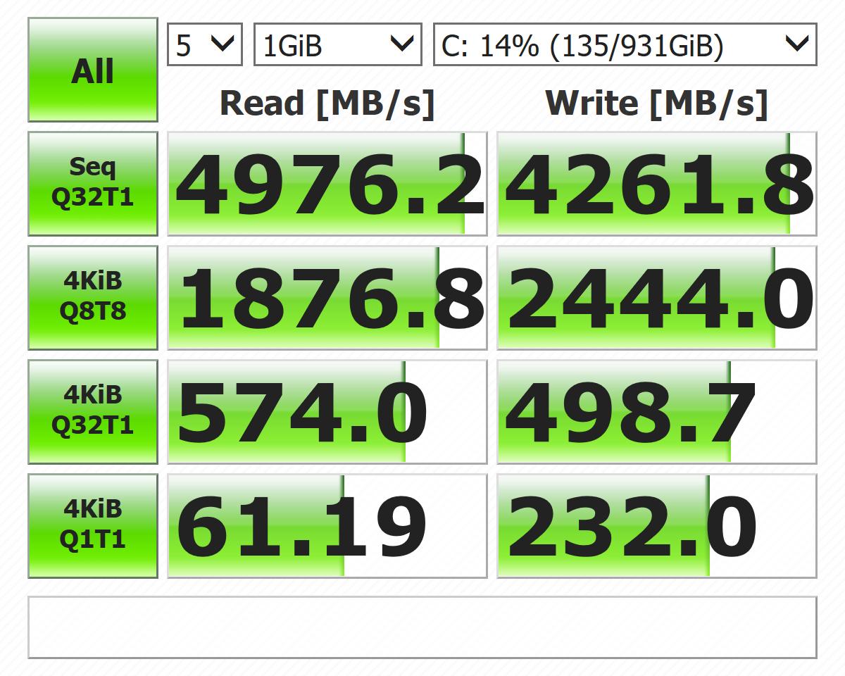
For various reasons (including that while Linux is a fantastic OS in lots of regards, it still sucks on the desktop, especially for my particular needs) I loaded up Windows 10. CrystalDiskMark is a good free benchmark and I was able to test my new NVMe drive there.
I ran it, thinking I’d get the same results from Linux. Nope!
I got pretty much what the drive promised.
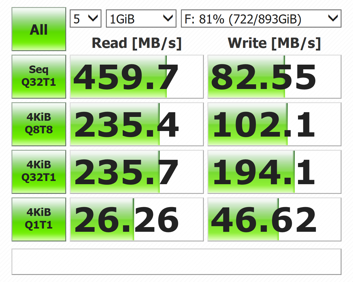
As a comparison, here’s how my old SATA SSD fared:
About 10x performance. Here’s a couple of takeaways:
PCIe 4 does matter for storage throughput. Would I actually notice in my day-to-day operations the difference between PCIe 3 and PCIe 4? Probably not. But I’m working with 4K video and some people are already working with 6K and even 8K video, that’s not too far down the line for me.
SATA is dead for SSD storage. The new drives are more than capable of utterly overwhelming SATA 3 (600 MB/s, LOL). Right now, SATA is sufficient for HDDs, but as platters get bigger sequential reads will continue to climb.
I don’t doubt that Linux can do the same, it’s just my methodology failed me. The dd command from /dev/zero had never failed to be the best way to test write speeds for HDD and SATA SSDs, but now I need to find another method for Linux (or perhaps there is some type of bottleneck in Linux).
TL;DR
New PCIe 4 NVMe SSDs are super fast and can be had for a relatively low amount of money ($180 USD for 1 TB). They’re insanely fast.